From Periodic Orbits to the Complex Dynamics of Turbulent Flow

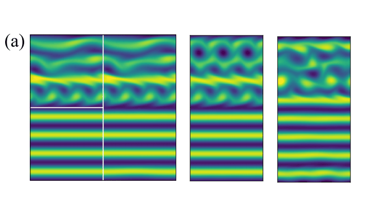
When dye enters moving water, it stretches into thin filaments, bends, and swirls, making the flow’s vortical motions visible. Gradually, its initial pattern becomes almost unrecognizable. Measuring the fluid’s velocity at different points makes it possible to track how the entire flow changes over time. But amid these continuous changes, can there be motions that repeat according to a particular rule?

Researchers have long sought recurrent solutions to the equations of fluid motion. In these solutions, the flow returns to its earlier pattern of motion after a certain time, sometimes with a particular spatial shift. Such motions are usually unstable: a trajectory that starts very close to them gradually moves away. Yet a chaotic flow can approach one of these recurrent solutions for a time.

Dmitriy Zhigunov and Jacob Page, mathematicians at the University of Edinburgh in the United Kingdom, investigated whether complex states of turbulent fluid flow could be built from recurrent motions previously computed for small domains. They examined how these motions interact within a shared flow and under what conditions individual regions can retain their own dynamics. Their computations yielded consistent solutions for an enlarged domain and examples in which motion in one part of the flow follows a known periodic orbit for a time.

To study recurrent motions, researchers use the concept of state space. In this space, the entire flow is represented by a single point whose position is determined by the distribution of fluid velocities. For their computations, Zhigunov and Page used a grid of 128 $\times$ 256 points. Two velocity components, horizontal and vertical, are accounted for at each point. In total, this amounts to about 65,000 numerical values linked by the equations of fluid motion.

As the flow changes, the point moves through state space, tracing a trajectory. If the entire velocity field repeats after a given time, this trajectory closes on itself. If the repetition involves a spatial shift, a closed cycle is obtained after accounting for the corresponding symmetry. The trajectory of a chaotic flow is much more complex, but it sometimes passes near such recurrent motions.

The instability of a recurrent motion is like that of a ball on a mountain ridge. Along the ridge, the ball may approach a saddle, while a small sideways displacement will send it down the slope. Recurrent solutions of the equations of fluid motion can likewise have directions along which nearby states approach the orbit and directions along which they move away from it. If a chaotic trajectory passes close enough to such an orbit, it can follow it for a time, until the deviations grow.

The approach of studying chaotic dynamics through recurrent solutions to the equations of motion was developed in earlier research. In their papers from 2022 and 2026, Predrag Cvitanović and Han Liang considered spatiotemporal chaos as a pattern assembled from simple recurrent solutions. In 2001, Genta Kawahara and Shigeo Kida discovered periodic motion within a model of turbulent shear flow. Later, Chandler and Kerswell computed recurrent solutions for two-dimensional Kolmogorov flow. In 2017, Balachandra Suri and colleagues found experimentally that flow in a thin fluid layer can approach unstable steady states. They also studied how the flow then departs from those states. In 2020, Suri and colleagues demonstrated experimentally that a turbulent flow can temporarily shadow unstable periodic orbits. In 2024, Jacob Page’s group used a set of orbits to reconstruct the flow’s statistical properties. Zhigunov and Page’s study extends this approach to an enlarged computational domain, where neighboring parts of the flow can move differently.

Why Combining Motions Requires a Consistent Solution

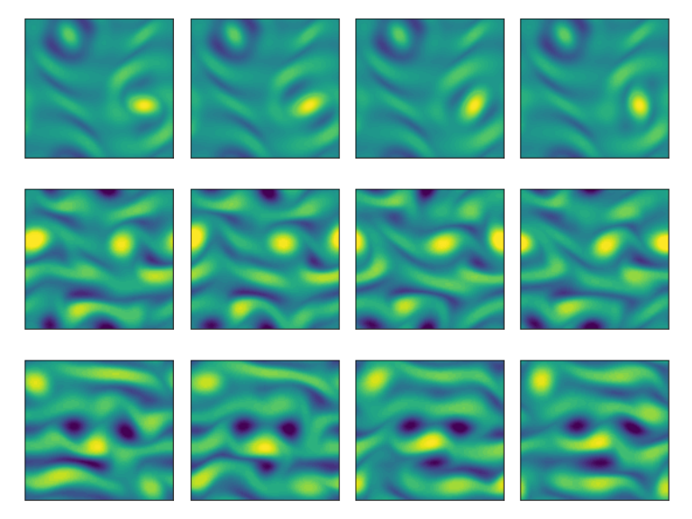
Fluid motion is described by the Navier–Stokes equations. They account for changes in velocity as well as pressure, viscosity, and external forces. The fluid velocity in one part of a flow depends on the motion of neighboring parts. A change in the flow at one location can therefore affect the rest. If a vortical motion is placed next to a calm laminar flow, the resulting field will generally no longer be a solution to the equations for the entire enlarged domain. The situation is different when the same periodic field is repeated in neighboring cells: such an extension can satisfy the original equations exactly.

To investigate interactions between different fluid motions, Zhigunov and Page chose a mathematical model of two-dimensional Kolmogorov flow. In this model, an external force acts horizontally, reversing direction periodically along the vertical axis. Opposite edges of the computational rectangle are mathematically connected: a field crossing one boundary continues from the opposite side (periodic boundary conditions). The researchers fixed the Reynolds number at Re = 40. It characterizes the relative importance of inertia and viscosity at the chosen length and velocity scales. The study concerns relatively weak turbulence in a two-dimensional model. Many natural and engineering flows have much higher Reynolds numbers; their values also depend on the velocity and length scales used in the calculation.

In nondimensional form, the equations are:

$\partial_t u$ + ($u\cdot\nabla$)$u$ = −$\nabla p$ + (1/Re) $\Delta$u + eₓ sin(4y),

$\nabla\cdot u$ = 0

Here, $u$ is the fluid velocity at each point, and $p$ is pressure. The term $\partial_t u$ describes the change in velocity over time, while ($u\cdot\nabla$)$u$ describes the change due to advection by the flow. The expression −$\nabla p$ describes the effect of pressure differences, and (1/Re) $\Delta$u describes the effect of viscosity, which smooths out velocity differences. The external force eₓ sin(4y) acts along the horizontal $x$ axis and changes sign periodically with the coordinate $y$. The condition $\nabla\cdot u$ = 0 expresses incompressibility: the volume of a small fluid parcel is conserved. These equations determine how a given initial state evolves, but complex recurrent solutions must be sought using specialized computational methods.

As their starting set, the researchers used a library of relative periodic orbits: solutions in which the velocity field repeats after a certain time once a spatial shift is taken into account. These orbits had previously been computed for a 2$\pi \times$ 2$\pi$ domain, including in the 2025 study by Andrew Cleary and Jacob Page. The authors made the new domain twice as tall while keeping the same width: 2$\pi \times$ 4$\pi$. With the chosen external force, the small square contains four wavelengths of the forcing, and the large rectangle contains eight. Two small squares can be stacked vertically; to obtain a single solution for the enlarged domain, the interaction between the flows in these squares must be taken into account.

Recurrence with a Shift

Before recurrent motions can be joined, it is necessary to specify what kind of return counts as a recurrence. Sometimes, after a time $T$, the vortices return to their earlier arrangement relative to one another, but the entire pattern has shifted horizontally. If the whole velocity field matches after accounting for this shift, researchers call the motion a relative periodic orbit (RPO). This condition is expressed by the formula:

$u(x, y, t + T)$ = $u(x + \delta, y, t)$

The left-hand side gives the velocity field after a time $T$; the right-hand side gives the field at the initial time, evaluated with a horizontal shift $\delta$. The letters $x$ and $y$ denote the coordinates of a point, and t denotes time. The sign of $\delta$ depends on the convention used to define the direction. Numerically, this means determining the initial velocity field, which specifies the trajectory, together with the return time $T$ and the spatial shift $\delta$.

Because such orbits are usually unstable, starting a standard simulation from nearly the same initial state may soon lead to a different flow. Zhigunov and Page needed a specialized procedure that finds the motion and then quantitatively checks how closely it returns to its initial state after the period and shift.

How to Join Two Regions of Fluid

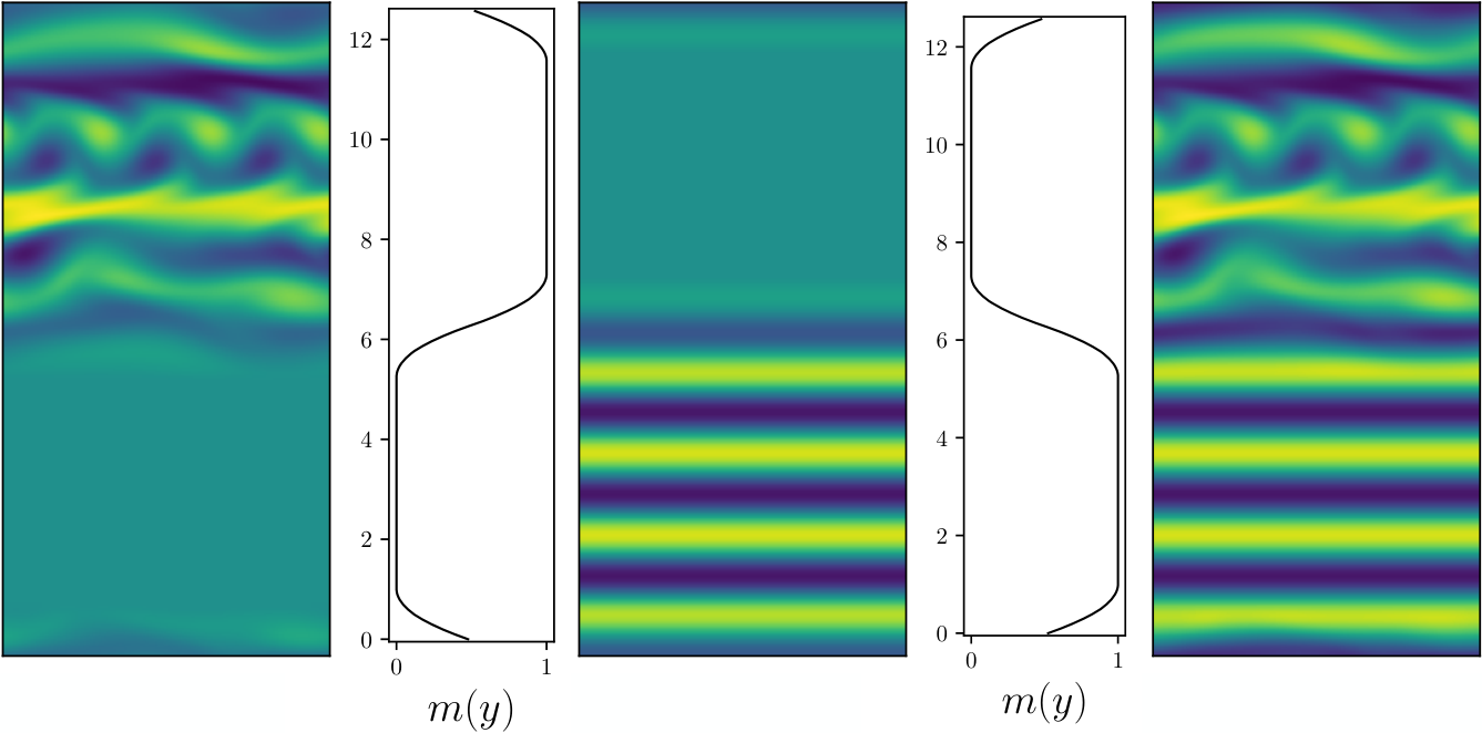
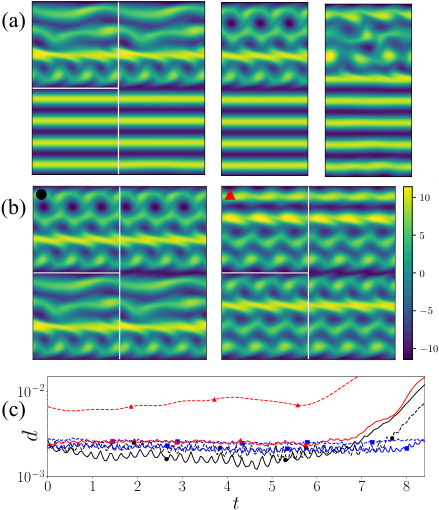
The researchers began with one of the orbits previously computed for the small square. They placed its velocity field in one half of the enlarged rectangle and a calm laminar flow, with velocities arranged in orderly layers, in the other. The laminar state satisfies the chosen equations under the same external force. The initial fields were joined using smoothing weight functions to produce an initial guess for a subsequent numerical procedure that makes the motion consistent across the entire domain.

To do this, the authors numerically refined the entire velocity field. In the first stage, optimization reduced the difference between the state after the trial period and the initial field, taking the horizontal shift into account. The Newton–Krylov method, designed to solve large systems of nonlinear equations, then refined the resulting approximation to high accuracy. The authors thus obtained a single numerical solution for the enlarged domain that satisfied the Navier–Stokes equations to very high numerical accuracy.

For the 25 full-domain relative periodic orbits, recurrence of the velocity field was checked throughout the domain. Later, in the search for two-frequency motions and local shadowing, the researchers used a spatial mask: it allowed them to compare motion only within a selected region, even though the equations were solved over the entire domain.

For example, when searching for local shadowing, the researchers assessed how closely the velocity field in one half of the domain returned to its earlier state after a chosen time, accounting for a horizontal shift. They did not require the other half to exhibit the same recurrence, although the two parts of the flow continued to interact and their motion was computed together. A full-domain relative periodic orbit, by contrast, required the entire velocity field to recur, rather than just part of it.

After the final numerical refinement, the authors obtained 25 relative periodic orbits with a relative residual below $10^{-10}$. Here, the residual measures the relative difference between the initial field and the field after one period, accounting for the shift. This result means that the recurrence condition is satisfied numerically to very high accuracy.

Why a Calm Region Does Not Always Disrupt Vortices

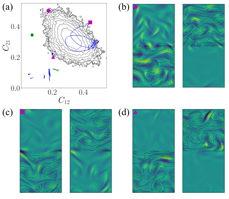
Joining two motions was easier where their interaction was weak. Vorticity in one part of a two-dimensional flow produces a velocity field beyond that region as well. But several closely spaced vortices of opposite signs can partially cancel one another’s effects on a neighboring region. Zhigunov and Page observed such groups of intense vortices and described this as a shielding effect. Even strong vortices can therefore have a relatively weak influence on a neighboring part of the flow. Weak interaction between neighboring regions makes it easier to find a combined motion that satisfies the equations to high numerical accuracy.

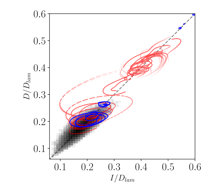
The researchers divided the vorticity field into two parts and assessed how strongly they affected each other. To do this, they compared the contributions of vortices in a region and in its neighboring region to vorticity advection. If the neighboring region’s share of the influence was less than 0.5, the local vortices’ influence dominated. When analyzing a long turbulent trajectory, the authors also varied the position of the boundary between the regions, choosing the partition that minimized their interaction.

With the partition chosen by the authors, the normalized share of the neighboring region’s influence was most often around 0.35 for each half of the flow. Each half’s own motion generally dominated, but coupling between the halves remained. For most of the 25 periodic orbits found, the influence of neighboring regions was even weaker than in typical turbulent states. In the coupling-coefficient diagram, most of these orbits lay far from the region frequently visited by the long turbulent trajectory.

When Neighboring Regions of a Flow Have Different Periods

After combining a periodic orbit with a laminar patch, the authors tested a more complex case: two different recurrent motions in neighboring halves of the domain. Each region has its own period and horizontal shift. When the two periods are incommensurate, the combined motion can no longer be described by a single cycle. It is called two-frequency, or quasiperiodic, motion. In state space, such two-frequency motion may correspond to a geometric structure called a two-dimensional invariant torus (a two-torus). The authors searched for numerical trajectories resembling this kind of motion.

A torus is usually depicted as the surface of a doughnut. Here, it is a geometric object in state space: two independent phases describe motion in two directions along this surface, with one phase for each frequency. The fluid itself remains in the rectangular computational domain. The presence of two frequencies in a computed trajectory provides a reason to look for such a torus.

For each half of the domain, the researchers separately determined a period and a horizontal shift after which its velocity field was close to its initial state. Their criterion was the relative recurrence residual $\varepsilon_i$, calculated after masking the selected region. As optimization progressed, they progressively lengthened the integration interval. For six trajectories, they reduced the residual in each half to no more than 1% when checking recurrence over at least two of that half’s own periods.

The researchers separately checked how close the motion in each half of the domain remained to its corresponding original orbit between recurrence times. For this, they used the distance $d_i$(t), accounting for shift and phase. The model’s characteristic Lyapunov time was about two nondimensional units: over such an interval, small differences between states grow appreciably. On some trajectories, proximity to the original orbits persisted for several such intervals.

In the first six cases found, the interaction between the two halves of the flow was particularly weak. In addition to these first six trajectories, considered candidates for two-frequency motion, the researchers obtained five more such candidates, bringing the total to eleven. In diagrams showing interactions between parts of the flow, energy input, and viscous dissipation, these five candidates fell within regions characteristic of long-term turbulent dynamics.

When Recurrence Appears in Only Part of the Flow

The authors separately investigated local shadowing: cases in which motion in one part of the flow remains close to a known periodic orbit for a time, while the motion in a neighboring region evolves in a much more complex way. To find such cases, the researchers optimized numerical trajectories and compared velocity fields in the selected half of the computational domain with the corresponding states of the original orbit. At each instant, they assessed closeness using the distance d(t) between the state of the selected flow region and a state on the original orbit matched by phase and horizontal shift.

The researchers used 21 small-domain orbits and obtained 32 specifically optimized local shadowing trajectories; these trajectories corresponded to 16 orbits from the initial set. Along these 32 trajectories, the distance d(t) remained no greater than 1% for more than two full periods of the corresponding original orbit. Outside the selected region, the motion could remain chaotic. The number 32 refers to local episodes and is not added to the 25 periodic orbits computed to high numerical accuracy.

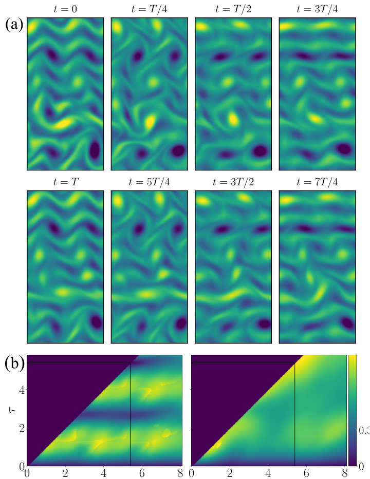
Because these 32 trajectories were specifically constructed through optimization, their number cannot be used to infer how often local shadowing occurs in a freely evolving flow. In the supplemental material, the authors note that unphysical features of the optimized initial fields quickly smoothed out as the flow evolved further, after which local shadowing was observed.

The Limits of the Results Established So Far

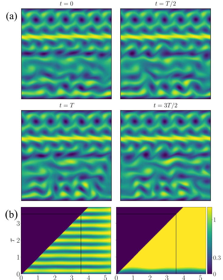
To study interactions between different motions in neighboring parts of a flow, Zhigunov and Page used a two-dimensional model of Kolmogorov flow with periodic boundary conditions, a sinusoidal external force, and a Reynolds number of Re = 40. They also tested local shadowing in a larger two-dimensional domain, 4$\pi \times$ 4$\pi$, and had found four numerical examples by the time of publication, one of which is shown in Figure 7.

This model has limitations, however. In three-dimensional flows, vortex stretching can occur; this mechanism is absent in the two-dimensional model. Pipe and channel walls can also affect fluid motion, but their effects were not included in the authors’ computations.

Zhigunov and Page showed how recurrent solutions computed for small domains can be used to build more complex states of a two-dimensional flow. They obtained 25 relative periodic orbits, found 11 candidates for two-frequency structures, and computed 32 local shadowing trajectories.

These results differ in how firmly they are established: the relative periodic orbits were computed to high accuracy, the two-frequency structures are considered candidates, and the local shadowing trajectories were obtained through specialized optimization. The authors published the code and numerical data in the University of Edinburgh’s data repository, allowing other researchers to check the computations independently and extend the work.

The numerical results show that interacting regions with different dynamics can coexist within a single flow. When their mutual influence is relatively weak, motion in one part of the flow can remain close to a known periodic orbit for several periods, while much more complex dynamics develop in a neighboring region. The proposed method makes it possible to construct and study local shadowing trajectories without requiring the flow to be periodic throughout the computational domain.