A Random Graph Sandwich: Proof Twenty Years Later

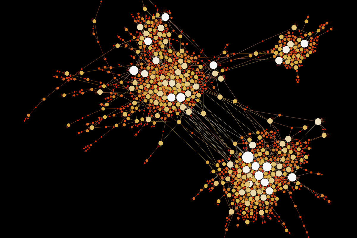
Each of the four panels shows twenty points, with lines connecting some pairs. Even a diagram like this allows us to ask rigorous questions about a network. In graph theory, the points are called vertices, and the lines connecting them are called edges: an edge represents a connection between two vertices. The entire structure is called a graph. It retains information about connections: which vertices are connected to one another and which connections are absent. This language suits a wide range of problems, such as routes between stations or connections between computers, when the researcher is interested in the structure of a network.

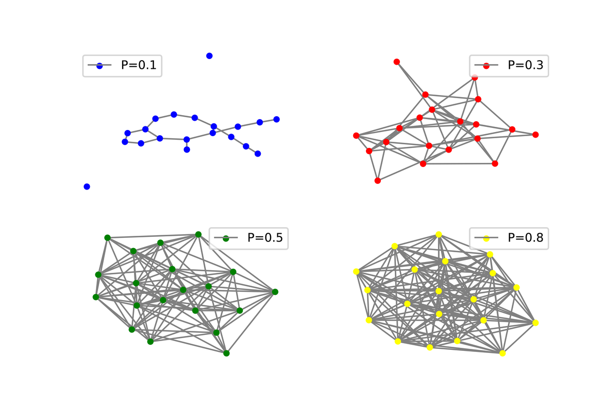
As the number of vertices grows, there are too many possible graphs to examine them all. We then specify a rule for constructing a graph at random and ask which properties will occur almost always under that rule. In random graph theory, the expression “with high probability” means precisely this: as the number of vertices grows, the probability of the property tends to one. For example, we might ask whether it is possible to follow connections from any point in the network to any other, or whether there is a closed route that visits every point exactly once. In their 2004 paper “Sandwiching random graphs: universality between random graph models,” mathematicians Jeong Han Kim and Van H. Vu compared two ways of constructing a random graph. In the first, each possible connection appears independently of the others. In the second, the final graph must have the same number of edges at every vertex. Both rules can produce graphs with approximately the same total number of connections, although the dependence between individual edges differs.

A wealth of theorems and probabilistic techniques has been developed for the model with independent edges. In the model with the same number of edges at each vertex, adding an edge immediately gives two vertices one additional connection each and changes the remaining possibilities for both. Kim and Vu proposed linking the two models through graph containment. Their idea was to place a graph with the same number of edges at every vertex between two graphs with independent edges: one with slightly fewer connections on average, the other with slightly more. The result is a kind of sandwich: the edges of the lower graph belong to the middle graph, and the edges of the middle graph belong to the upper graph. This containment allows some results about the independent-edge model to be transferred to the graph in the middle of the sandwich.

Kim and Vu formulated this idea as the sandwich conjecture. Its statement was brief, but the path to a complete proof took about twenty years. In 2025, the conjecture was proved by Natalie Behague, Daniel Iľkovič, and Richard Montgomery, mathematicians at the University of Warwick’s Mathematics Institute; Iľkovič is also affiliated with Leipzig University. Montgomery announced the result in September 2025 at an international workshop on combinatorics and probabilistic methods at the Oberwolfach Research Institute for Mathematics in Germany. The preprint was posted on arXiv on October 23, 2025, and a second version appeared on December 8, 2025. In an interview published by Quanta Magazine on September 18, 2026, about a year after the announcement, Natalie Behague described the connection between the two models as “almost too good to be true.”

To understand why establishing this connection proved so difficult, we need to take a closer look at how the two random graph models work. At first glance, they seem similar: both can produce graphs with approximately the same number of edges. But the rules governing how those edges appear differ substantially.

Two Random Graph Models

Let a graph have $n$ vertices. The letter $n$ denotes their number. One standard model is written as $G(n,p)$ and is called the binomial model (it is also known as the Erdős–Rényi random graph model). For each pair of vertices, a separate decision determines whether an edge will appear between them. The probability that an edge appears is denoted by $p$. The choice for one pair does not change the probability for any other pair. Consider a single vertex. Apart from that vertex, there are $n-1$ other vertices in the graph, and a connection to each can appear with probability $p$. The number of edges at a particular vertex is therefore not fixed in advance: by chance, one vertex may have slightly more and another slightly fewer. The expected degree of a vertex is exactly $(n-1)p$. In the second model, this number is fixed in advance. The Petersen graph in the next figure helps show what this changes.

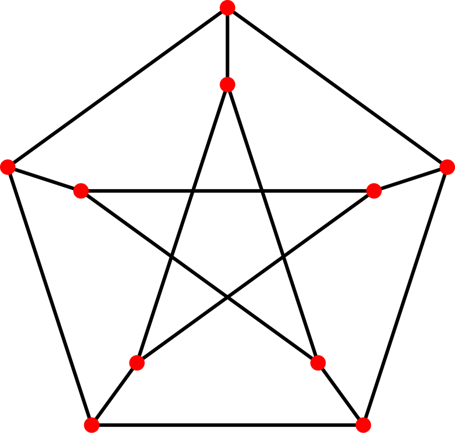
In the Petersen graph, exactly three edges meet at each vertex. Two vertices joined by an edge are considered neighbors: each point in the diagram has three neighbors. The number of neighbors of a vertex is its degree. If every vertex has the same degree, the graph is called regular, and this common degree is denoted by $d$. For the Petersen graph, $d=3$. The notation $G_d(n)$ denotes a uniformly random $d$-regular graph on $n$ labeled vertices. The product $nd$ must be even, since the sum of vertex degrees counts every edge twice. If such a graph has degree 3 and a vertex already has three neighbors, a fourth edge cannot be added to it. A new edge gives two vertices one additional neighbor each and immediately reduces the number of connections that can still be added at either vertex.

Having the same number of edges at each vertex describes only the immediate connections; the structure of the network as a whole remains a separate question. In the Petersen graph, it is impossible to follow edges through all ten vertices exactly once and return to the starting point. Such a closed route is called a Hamiltonian cycle. For random regular graphs, an important question is how often properties of this kind arise as $n$ grows.

Dependence between edges also makes constructing a random regular graph more difficult. We cannot simply add connections at random: some vertices may reach their allotted $d$ neighbors too early, leaving no suitable connections for the others. Even completing the graph is not enough. Every admissible $d$-regular graph must be produced with the same probability; otherwise, the random selection will be biased. In the $G(n,p)$ model, things are simpler: each possible edge appears independently with probability $p$, and there is no imposed limit on the number of neighbors a vertex may have. In a regular graph, choosing one edge affects which edges can be added next.

How Three Graphs Form a Sandwich

The Kim–Vu sandwich uses the same set of $n$ vertices. In the middle is a random $d$-regular graph $G$. The lower graph $G_*$ has slightly fewer edges on average, and the upper graph $G^*$ slightly more; both follow the binomial rule, in which edges are chosen independently. In general, constructing the three graphs independently does not ensure the required containment. To obtain that containment while preserving each graph’s distribution, the three constructions are linked through a shared random mechanism. In probability theory, this kind of joint construction is called a coupling; we will use that term below.

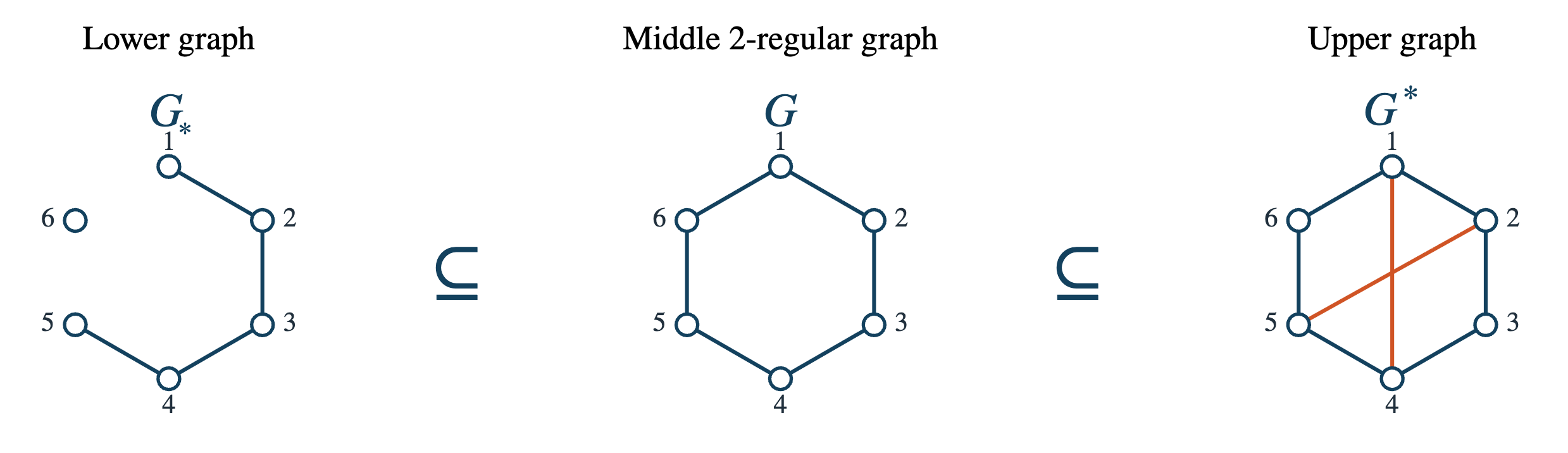
The diagram below shows three layers on the same vertex set. The regular graph $G$ is in the center, flanked by two binomial graphs with independent edges. The lower layer is slightly sparser than the central one, and the upper layer is slightly denser.

$$G_* \subseteq G \subseteq G^*$$.

The symbol $\subseteq$ means that every edge of the graph on the left belongs to the graph on the right. In the joint construction, the marginal distribution of $G$ must remain that of a uniformly chosen $d$-regular graph, and the outer layers must retain their binomial distributions. This is precisely the difficulty of coupling: the three graphs must be arranged in relation to one another without distorting the rules governing their random selection.

The outer graphs must have nearly the same number of connections as the regular graph. A graph’s density is the fraction of all possible pairs of vertices that are actually connected by an edge; in the binomial model, its expected value is given by the probability $p$. In the regular graph, every vertex has exactly $d$ neighbors. In $G(n,p)$, a vertex has exactly $(n-1)p$ edges on average; for large $n$, this is close to $np$. Choosing $p \approx d/n$ therefore gives the same scale for the number of connections. The lower probability $p_*$ is chosen slightly below $d/n$, and the upper probability $p^*$ slightly above it. The smaller the relative difference between them, the closer the outer graphs are to the regular graph. Formally:

$$G_* \sim G(n,p_*), \quad G \sim G_d(n), \quad G^* \sim G(n,p^*)$$,

$$p_* = (1-o(1))d/n, \quad p^* = (1+o(1))d/n$$,

$$\Pr(G_* \subseteq G \subseteq G^*) = 1-o(1)$$.

The first line specifies the distribution of each of the three graphs. Here, the symbol $\sim$ means “has this distribution,” and $\Pr$ denotes the probability of the event in parentheses. The notation $o(1)$ denotes a quantity that tends to zero as $n$ grows. Thus, $p_*$ and $p^*$ bracket $d/n$ ever more closely, and the probability of the containment $G_* \subseteq G \subseteq G^*$ tends to one. The larger $n$ becomes, the thinner the sandwich becomes relative to its own scale.

Why This Containment Matters in Mathematics

The usefulness of the sandwich is easiest to see for properties that are preserved when edges are added. Take connectivity. If we can follow a chain of edges from any vertex to any other, the graph is called connected, and this property is called connectivity. Adding new edges does not destroy existing paths. A Hamiltonian cycle behaves the same way: additional connections do not interfere with a closed route that visits every vertex. In random graph theory, such properties are called monotone increasing: once they hold, they continue to hold as edges are added.

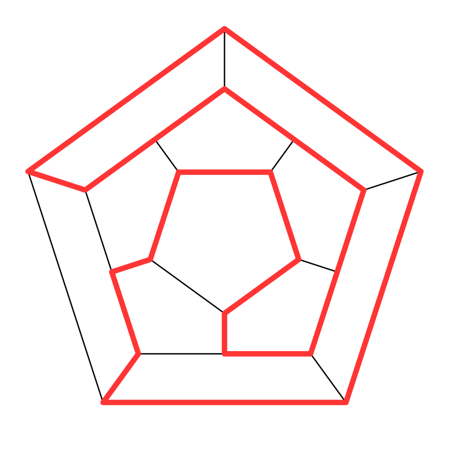
Suppose that such a property has been proved to hold with high probability for the lower binomial graph $G_*$. All its edges belong to the regular graph $G$, so an existing route or connectivity is preserved in $G$ as well. In this way, a result from the simpler model $G(n,p)$ transfers to a random regular graph. The upper inclusion $G \subseteq G^*$ provides control over properties of a different kind. For example, if the upper graph admits a proper coloring with $k$ colors, the same coloring works for $G$ after the extra edges are removed. Here, colors are simply labels assigned to vertices; vertices joined by an edge must have different labels. In an application, such a label might represent a frequency, a time slot, or another resource that cannot be assigned simultaneously to connected objects.

Inclusion alone transfers only properties that are guaranteed to survive the addition or deletion of edges. For some problems, this is enough; for others, the precise point at which a property appears matters. Imagine that, as $p$ increases, a property initially occurs rarely and then becomes almost inevitable within a narrow range of $p$. This region of rapid transition is called a threshold window. There is also a limit to how sparse the sandwich can be: the outer layers must remain dense enough for the regular graph to fit between them.

Where the Logarithmic Boundary Comes From

The theorem of Behague, Iľkovič, and Montgomery places a natural restriction on the degree $d$. The upper binomial graph can contain a $d$-regular graph only if each of its vertices has at least $d$ neighbors. In $G(n,p)$, the number of connections at different vertices fluctuates randomly around the mean. When the graph is too sparse, with high probability at least one of its many vertices will have fewer than $d$ neighbors; a $d$-regular graph then cannot fit inside the upper layer. For a sandwich with a vanishingly small relative gap, this obstacle disappears when $d$ grows faster than $\log n$. This condition is written as follows:

$$d = \omega(\log n), \quad \text{that is,} \quad d/\log n \to \infty$$.

The notation $d/\log n \to \infty$ means that, as $n$ grows, $d$ becomes arbitrarily many times larger than $\log n$; the symbol $\omega$ in $d = \omega(\log n)$ expresses the same asymptotic relation. The quantitative statement of the theorem also includes the condition $d \ge C \log n$. Here, $C$ is a fixed positive constant: a number chosen sufficiently large depending on $\varepsilon$, the allowed relative deviation of each outer edge probability from $d/n$, and then held fixed as $n$ grows. This dependence is written as $C = C(\varepsilon)$. For any fixed $\varepsilon > 0$, the condition $d \ge C(\varepsilon) \log n$ is sufficient; a relative error tending to zero requires $d/\log n \to \infty$.

Why the Complete Proof Took Twenty Years

Proving the existence of the full sandwich for degrees $d$ only slightly above the logarithmic scale proved difficult. Mathematicians gradually expanded the range of $d$ for which they could establish the required inclusions between random graphs. In their original paper, Kim and Vu proved the lower inclusion over part of the range and obtained a weakened version of the upper inclusion. In 2017, another group of mathematicians, Dudek, Frieze, Ruciński, and Šileikis, extended the range in which the lower inclusion holds. Pu Gao, Mikhail Isaev, and Brendan McKay then obtained the first full sandwich for denser random regular graphs and later reached the regime $d \gg \log^4 n$, that is, $d/(\log n)^4 \to \infty$. The notation $\log^4 n$ means $(\log n)^4$. The full conjecture requires a much sparser regime, where $d$ grows faster than $\log n$, that is, $d/\log n \to \infty$. Between $\log n$ and $\log^4 n$ lay a large range that the earlier analysis did not cover.

The hardest part remained the upper inclusion $G \subseteq G^*$. The upper binomial graph must be only slightly denser than the regular graph while retaining the exact distribution $G(n,p)$. Containment is not enough: the coupling must also preserve the prescribed distributions of all three graphs.

The coupling procedure was introduced in earlier work by Gao, Isaev, and McKay. The new proof develops its analysis through estimates for switching paths. These are paths whose edges alternate between a regular subgraph and additional edges in the current graph; they can be used to rearrange edges without changing vertex degrees. The method is explained below in the discussion of switching. The authors do not require the desired estimate for the number of such paths to hold for every possible $d$-regular subgraph. The main switching result allows a very small fraction of exceptions: at most $n^{-6}$ of all $d$-regular subgraphs contained in the graph under consideration. This bound applies specifically to the fraction of exceptions within that family, rather than to the overall probability that the sandwich construction fails. The authors obtain the required accuracy for typical graphs; they retain the small exceptional group in the calculation and show separately that its contribution does not change the overall result.

Two Coupling Processes

Imagine that several edges have already been selected, forming an unfinished diagram. It still needs to be completed to a $d$-regular graph in which every vertex has exactly $d$ neighbors. We will call the possible final graphs that contain all the edges already selected “regular completions.” When a new edge is proposed, the authors estimate how many such completions will remain if it is accepted. An edge that reduces the number of possible completions too sharply is given a lower chance of being accepted.

The final graph must still be sampled uniformly. While constructing the unfinished graph $F$, the authors also build an auxiliary random graph. When the next edge is considered, the same fresh random number $u$, sampled uniformly from $[0, 1]$ independently of earlier trials, is used for both graphs, but it is compared with different acceptance thresholds. If the threshold in the auxiliary process is lower, an edge accepted there must also be included in $F$. This ordering of the thresholds, however, cannot be assumed to hold at every step. The authors prove that, with high probability, it holds throughout the required portion of the construction. The result is an auxiliary graph with a fixed number of edges, with every graph having that many edges equally likely. This graph is then coupled in a further step with the lower binomial layer $G_*$, in which edges appear independently of one another. In this way, the main goal is achieved with high probability: all the edges of $G_*$ belong to the final regular graph $G$.

The upper process runs in the opposite direction. It begins with the complete graph, a network in which every pair of vertices is connected.

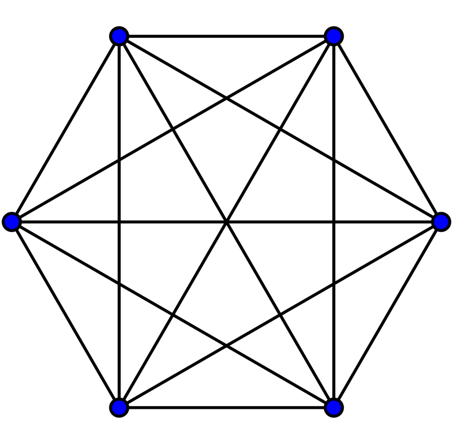
Edges are then proposed for deletion one at a time. After each deletion, the remaining network must still contain $d$-regular subgraphs on all the original vertices; we will call these subgraphs regular backbones. In graph theory, such spanning $d$-regular subgraphs are called $d$-factors. Before each step, the authors estimate how many backbones will survive. An edge whose deletion would destroy too many admissible backbones is given a lower chance of deletion. The probability of deleting a proposed edge $e$ is given by the formula:

$$a_e(F) = \frac{N_d(F - e)}{\max_{f \in E(F)} N_d(F - f)}$$.

Here $F$ is the current graph, $E(F)$ is its edge set, $F - e$ is obtained by deleting $e$, $N_d(H)$ is the number of spanning $d$-regular subgraphs of $H$, and $a_e(F)$ is the acceptance probability for deleting the proposed edge $e$. The formula compares how many admissible regular backbones remain after different possible deletions. The numerator is the number of backbones that survive the deletion of the particular edge $e$. The denominator is the largest such number among all edges that can be deleted at this step. At every step before the process stops, the denominator is positive and the ratio lies between zero and one; it gives the probability of accepting the proposed deletion. If deleting $e$ would destroy all regular backbones, the numerator is zero, and the edge is retained. The current graph $F$ thus gradually loses edges until it becomes a $d$-regular graph $G$. The resulting $G$ has the required uniform distribution, while the upper binomial layer $G^*$ is obtained through an additional coupled construction.

The two coupling processes differ primarily in their number of steps. A $d$-regular graph has exactly $nd/2$ edges: each of the $n$ vertices has $d$ connections, and each edge has been counted twice, once at each end. The addition process must accept exactly $nd/2$ edges; more edges may be proposed, because some proposals are rejected. The complete graph contains $n(n-1)/2$ possible edges, a quantity of order $n^2$, so the deletion process can potentially involve far more steps. Even a small error in the probabilities can accumulate when repeated many times. The authors adjust the required accuracy as the process proceeds and control the total error.

Both processes produce a central $d$-regular graph with the same uniform distribution. This allows them to be combined into a single coupled construction sharing the same graph $G$. The addition process ensures $G_* \subseteq G$, and the deletion process ensures $G \subseteq G^*$. The failure probability for each part is bounded separately, and the bounds are then added. The overall probability of failure tends to zero.

Comparing Vast Numbers of Graphs Without Examining Them All

Deleting edges involves a subtlety: the choice of edge can substantially change the number of $d$-regular graphs that can still be obtained. If many such graphs remain after one edge is deleted but far fewer remain after another, coupling the deletions with the upper binomial layer will be difficult. The authors therefore need to show that these differences are small throughout the required portion of the process. The upper layer itself is constructed separately, according to a random rule that gives it a binomial distribution. Estimates of the number of regular backbones then allow the authors to prove that, with high probability, this layer contains every edge of the final regular graph. Counting all possible backbones directly is impossible: there are too many. Instead, the authors use a classical combinatorial technique called switching. It allows entire families of graphs to be compared without examining them all. The simplest form of such a switching is shown in the diagram below.

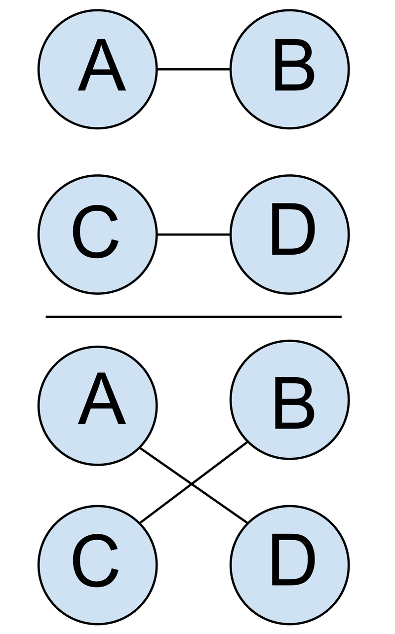
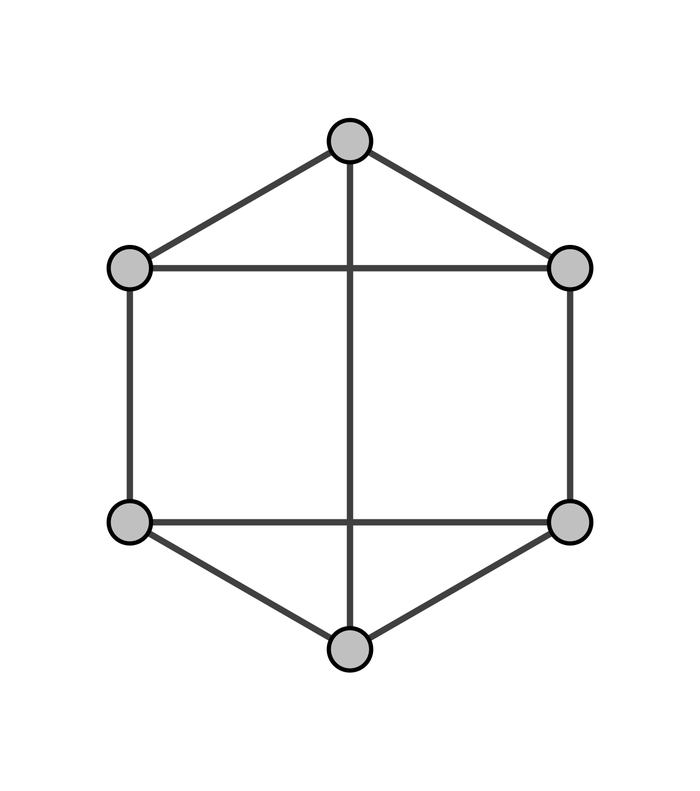
The four vertices in the diagram are labeled A, B, C, and D. Edges AB and CD are present in the original regular backbone. Connections AD and BC are allowed by the current graph $F$ but are not yet present in the backbone. If AB and CD are deleted and AD and BC are added, each of the four vertices loses one neighbor and immediately gains another. The number of neighbors at each vertex remains the same, while the regular graph itself changes. This exchange of edges is called a switching.

Switchings allow us to compare the sizes of large families: sets of graphs defined by a common condition. Choose two specific edges, $e$ and $f$. The first family consists of regular graphs in which $e$ is present and $f$ is absent; the second consists of graphs with the opposite arrangement of those two edges. An admissible switching takes a graph from the first family into the second. Each such transition can be counted from either side, because it connects exactly one graph in the first family with one graph in the second. If we know how many switchings are available on average from a graph in each family, we can estimate the ratio of the sizes of the two families, and then compare the probabilities that edges $e$ and $f$ are present.

A small numerical example shows how double counting works. Suppose the first family contains 100 graphs, each with four admissible switchings leading out of it. There are then 400 transitions between the families. If each graph in the second family has five reverse transitions, that family must contain 80 graphs, since $100 \times 4 = 80 \times 5$. In the actual proof, the exact numbers are not known in advance. The authors derive upper and lower bounds and separately control the rare graphs with unusually many switchings, so that a small group of exceptions does not distort the overall balance.

Why Short Switchings Are Sometimes Not Enough

The simplest switching uses four vertices and requires suitable connections nearby. In a sparse graph, the required parts may lie far apart. The authors then use longer alternating paths. Such a path starts with an extra edge of the current graph $F$ that does not belong to the regular backbone $K$, followed by a backbone edge, and then continues alternating between the two types. Two suitable paths can be joined into a cycle, and the roles of the edges along it can be exchanged. Each affected vertex loses one connection and gains one new connection; its number of neighbors is preserved.

To determine whether there are enough such paths for the switchings, we need to estimate their number. We will call the edges of the current graph $F$ that do not belong to the regular backbone $K$ extra edges. Suppose there are, on average, $\delta$ such edges at each vertex. The degree of the regular backbone is $d$. Starting from a chosen vertex, the first step along an extra edge offers approximately $\delta$ choices, and the next step along a backbone edge offers about $d$. Two successive steps give approximately $\delta d$ possible continuations. Repeating this pair of steps $\ell$ times gives the rough estimate $(\delta d)^{\ell}$. When the endpoints of these paths are distributed approximately uniformly over the $n$ vertices, any vertex chosen in advance receives roughly one out of every $n$ continuations. This gives the rough estimate:

$$(\delta d)^{\ell} / n$$.

The formula provides an initial estimate of the number of paths, after which the actual constraints are introduced into the calculation. A path must not return to a vertex it has already visited, some vertices may be forbidden at a particular step, and the two edge types must strictly alternate. Each of these conditions reduces the number of admissible routes. The authors need to prove that, after all these losses, enough paths remain to compare the required families of graphs.

Sparsity makes this count sensitive to small errors. At each step, the estimate of the number of possible continuations enters as a factor in the estimate of the total number of long paths. A small relative error is therefore repeated with each new step. If the number of continuations is overestimated by just 1% one hundred times in a row, the overall error factor becomes approximately $1.01^{100} \approx 2.7$. The authors therefore track the growth of the sets of vertices reachable in one, two, three, or more steps. In graph theory, such sets are called successive neighborhoods. Controlling them prevents local errors from accumulating to a level that would spoil the count. This is particularly difficult in the sparser regime: fewer admissible continuations remain, and a small relative error uses up the remaining margin more quickly.

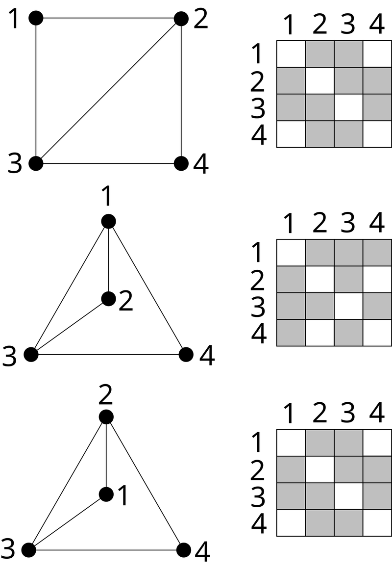
Once selected at random, a graph is fully specified: we know which edges it contains and which it does not. Its structure may nevertheless retain numerical features typical of the random model; such agreement with specified features typical of a random graph is called pseudorandomness. Earlier work controlled these features in part through the adjacency matrix. This is a table whose rows and columns correspond to vertices, with a 1 or 0 indicating whether a given pair is connected. The table yields spectral quantities, numbers that describe the distribution of connections across the graph as a whole. Behague, Iľkovič, and Montgomery work more directly with the construction itself: they study a random pair of graphs, count suitable paths directly, and show that rare exceptions do not change the overall scale of the count.

What the Proven Sandwich Makes Possible

The result of Behague, Iľkovič, and Montgomery links two random graph models almost down to the natural logarithmic boundary. For a fixed relative gap, their theorem already works when $d \ge C \log n$; if the gap must vanish as $n$ grows, the requirement is $d/\log n \to \infty$. A uniformly random $d$-regular graph can be coupled with two binomial graphs of nearly the same density so that $G_* \subseteq G \subseteq G^*$ holds with probability tending to one. This allows results on connectivity, Hamiltonian cycles, coloring, and other suitable properties proved for the well-studied $G(n,p)$ model to be transferred to random regular graphs through inclusion.

In July 2026, a paper by Mikhail Isaev and coauthors on the canonical labeling of random regular graphs received the best paper award for Track A at the ICALP conference. Canonical labeling makes it possible to recognize the same graph regardless of how its vertices are labeled or arranged. This work invokes the sandwich theorem of Behague, Iľkovič, and Montgomery to estimate edge counts between vertex sets in its treatment of dense random regular graphs. The new sandwich theorem applies for $d \ge C(\varepsilon) \log n$, with $\varepsilon$ controlling the relative error in each outer edge probability. This extends the earlier range $d \gg \log^4 n$, although the application just described uses the theorem in a dense regime.

In their paper, Behague, Iľkovič, and Montgomery also formulate the following conjecture. They propose coupling a single $d$-regular graph with an entire random process in which one randomly selected missing edge is added at each step. The process starts with $n$ isolated vertices and no edges; randomly chosen edges are then added one by one. The authors conjecture that, with high probability, the containment conditions will hold simultaneously at every step of this process. As long as the maximum number of neighbors of any vertex does not exceed $d$, the growing graph should fit inside the chosen $d$-regular graph. Once the minimum number of neighbors among all vertices reaches $d$, the reverse containment is expected: the $d$-regular graph should fit inside the growing graph. In their acknowledgments, the authors note that discussions at Oberwolfach led to this conjecture and suggested a simplification of the proof.

Unlike the already proven sandwich result, in which a regular graph is placed between two binomial random graphs, the new conjecture proposes that the required inclusions can be maintained throughout the entire process of random graph growth. This possibility remains unproven, and the authors note that establishing it will likely require fundamentally new ideas. Nevertheless, the proven sandwich result already makes it possible to apply findings from binomial random graphs to the study of random regular graphs almost down to the logarithmic threshold.

Sources

1. Behague, N., Iľkovič, D., & Montgomery, R. (2025, December 8). A proof of the Kim-Vu sandwich conjecture. arXiv preprint, arXiv:2510.20765v2 [math.CO]. https://arxiv.org/abs/2510.20765v2

2. Kim, J. H., & Vu, V. H. (2004). Sandwiching random graphs: Universality between random graph models. Advances in Mathematics, 188(2), 444–469. https://doi.org/10.1016/j.aim.2003.10.007

3. Dudek, A., Frieze, A., Ruciński, A., & Šileikis, M. (2017). Embedding the Erdős–Rényi hypergraph into the random regular hypergraph and Hamiltonicity. Journal of Combinatorial Theory, Series B, 122, 719–740. https://doi.org/10.1016/j.jctb.2016.09.003

4. Gao, P., Isaev, M., & McKay, B. D. (2022). Sandwiching dense random regular graphs between binomial random graphs. Probability Theory and Related Fields, 184(1–2), 115–158. https://doi.org/10.1007/s00440-022-01157-6

5. Gao, P., Isaev, M., & McKay, B. D. (2025, May 14). Kim–Vu’s sandwich conjecture is true for $d \gg \log^4 n$. arXiv preprint, arXiv:2011.09449v5 [math.CO]. https://arxiv.org/abs/2011.09449v5

6. Isaev, M., Makai, T., McKay, B. D., Prałat, P., Tan, J., & Zhukovskii, M. (2026). Canonical labelling of random regular graphs. In Proceedings of the 53rd International Colloquium on Automata, Languages, and Programming (ICALP 2026). Leibniz International Proceedings in Informatics (LIPIcs), Vol. 374, Article 114, pp. 114:1–114:23. https://doi.org/10.4230/LIPIcs.ICALP.2026.114

7. Montgomery, R. (2025). On the Kim–Vu sandwich conjecture (joint work with N. Behague and D. Iľkovič). In Combinatorics, Probability and Computing, Oberwolfach Report No. 42/2025, pp. 2287–2288. Workshop held September 14–19, 2025. DOI for the complete report: https://doi.org/10.4171/OWR/2025/42. Full report (PDF)

8. Rowińska, P. (2026, September 18). Mathematicians build long-awaited graph sandwich. Quanta Magazine. https://www.quantamagazine.org/mathematicians-build-long-awaited-graph-sandwich-20260918/

9. European Association for Theoretical Computer Science (EATCS). (2026). Best ICALP Paper: 2026 award recipients, Track A. https://eatcs.org/index.php/best-icalp-paper